The Mathematics of a Coin Toss

Why the dumbest game in the world explains almost everything that matters in markets

FINBEAR Observatory · Quantitative Foundations

First published September 2021. Rewritten from scratch July 27, 2026.

Opening note

We’re building QUANT, the area that will deliver a systematically selected set of stocks.

This article is here to help you read that list. Because there are two ways to receive it: as a promise — and then sooner or later it disappoints you — or knowing what a statistical edge actually is, how small it can be and still be real, and why nobody can tell you how the next toss will land.

It starts with a coin.

A coin has two sides. There is no poorer model than that, which is exactly why it’s the right place to start: when an object has one rule, everything that comes out of it has to come from the rule.

Out of that poverty come standard deviation, drift, Brownian motion, the Black-Scholes formula and — one step further on — the reason a portfolio can be right on average and die anyway.

The coin won’t tell you where the market goes tomorrow. It will tell you something less comfortable: that “where does it go tomorrow” is the wrong question.

Two Sides, and We’re Already Lost

One toss. Two outcomes:

\[S_1=\{H,T\}\]

If the coin is fair, each has probability 0.5. A single toss is a Bernoulli trial; counting how many Heads come up over N tosses takes us into the binomial distribution.

Two tosses give four sequences. Three give eight. Twelve give 4,096. A hundred tosses give:

\[2^{100} \approx 1.27 \times 10^{30}\]

A number roughly three trillion times larger than the number of seconds since the Big Bang.

One rule. No intent, no actor, no strategy. And the space of possible paths explodes to the point that no computer will ever enumerate them.

Hold on to that, because it’s the first working lesson here: the complexity you see on a chart is not evidence that somebody is behind it producing it. A few rules will do.

Building the Walk

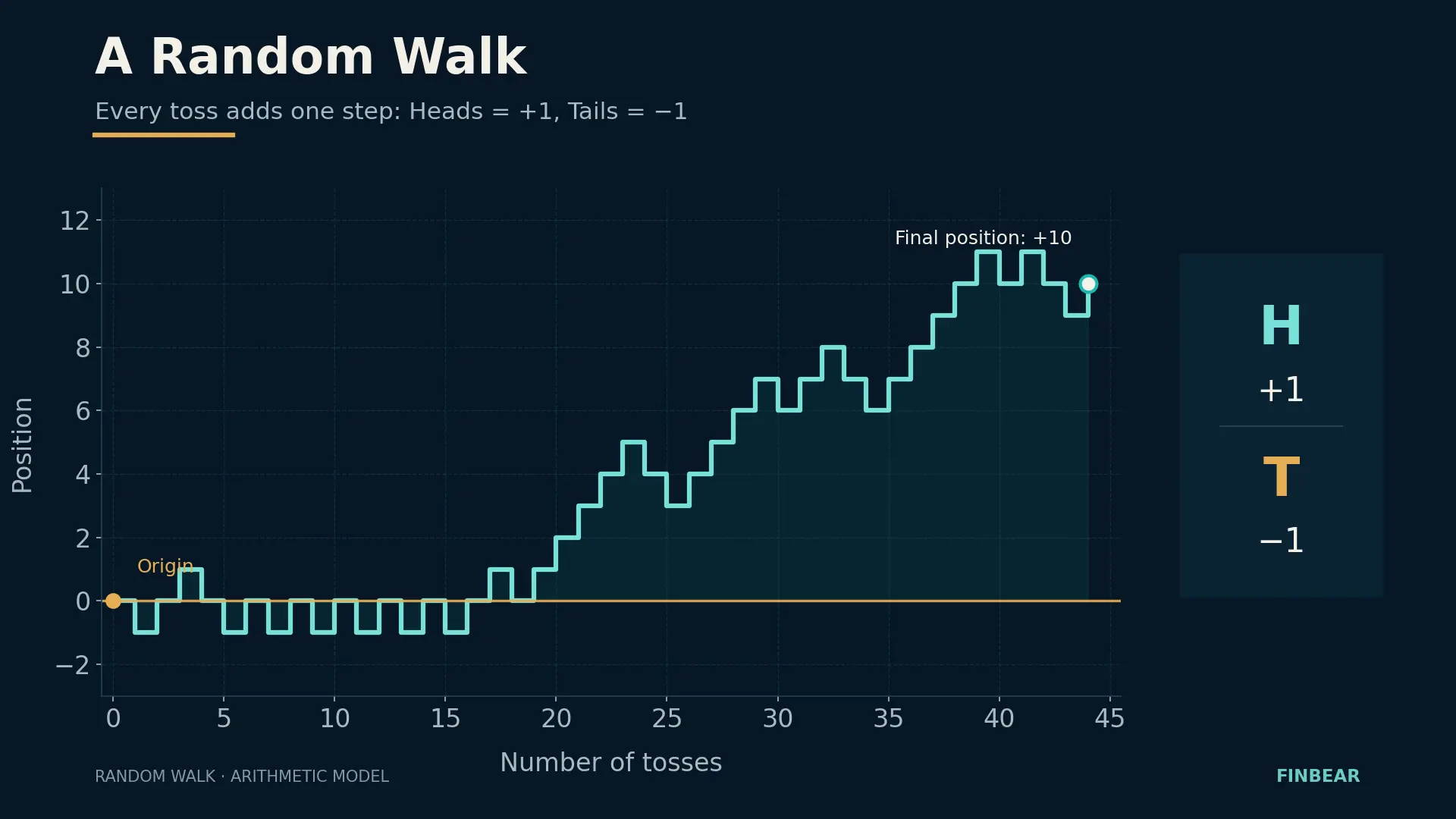
Assign a number to each outcome — Heads is +1, Tails is −1 — start at zero and toss N times. Your position after N tosses is the sum of the steps:

\[D_N = X_1 + X_2 + \dots + X_N\]

Each $X_i$ is only ever +1 or −1. The path rises, falls, climbs back, breaks lower. It draws a jagged line that, having decided nothing, looks a great deal like a price chart.

It’s called a random walk.

Expected Value Is Not a Forecast

For a fair coin, the expected value of one step is zero:

\[E(X) = (-1 \times 0.5) + (+1 \times 0.5) = 0\]

And therefore $E(D_N) = 0$.

This is where ninety percent of first-time readers go wrong, and they go wrong badly. Expected value of zero does not mean you’ll end at zero. It means the distribution of all possible endings is centered on zero. No individual path is obliged to pass through it.

Because while the center holds still, the width grows. For a fair coin:

\[Var(D_N) = N \qquad \sigma(D_N) = \sqrt{N}\]

After 100 tosses the standard deviation of the final position is 10 steps. After 10,000 tosses it’s 100 steps. The center hasn’t moved a millimeter; the uncertainty is ten times larger.

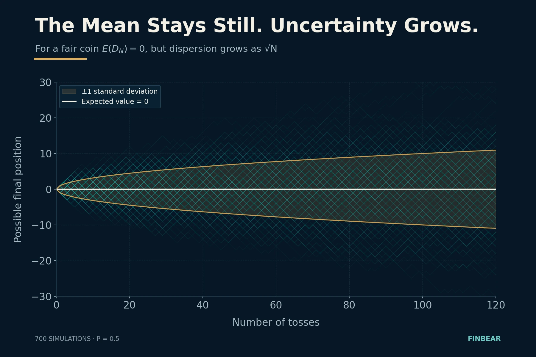
That’s the square root of time, and you’ll meet it everywhere: in annualizing volatility, in the width of bands, in any risk estimate over a horizon. One percent of daily volatility doesn’t make 252% a year — it makes about 16%, because $\sqrt{252} \approx 15.9$.

And here the lesson stops being mathematics and becomes craft.

A method with positive expected value can go through months of losses with nothing broken. A method with no edge at all can produce six excellent months on pure chance — and convince its author he’s a genius.

Being right isn’t enough. You have to survive the dispersion of results.

Anyone selling you a strategy by showing you the average has shown you half the problem. And he’s shown you the reassuring half.

What If the Coin Is Loaded?

Let Heads have probability $p$ and Tails $1-p$. The expected step becomes:

\[E(X) = p – (1-p) = 2p – 1\]

\[E(D_N) = N(2p-1)\]

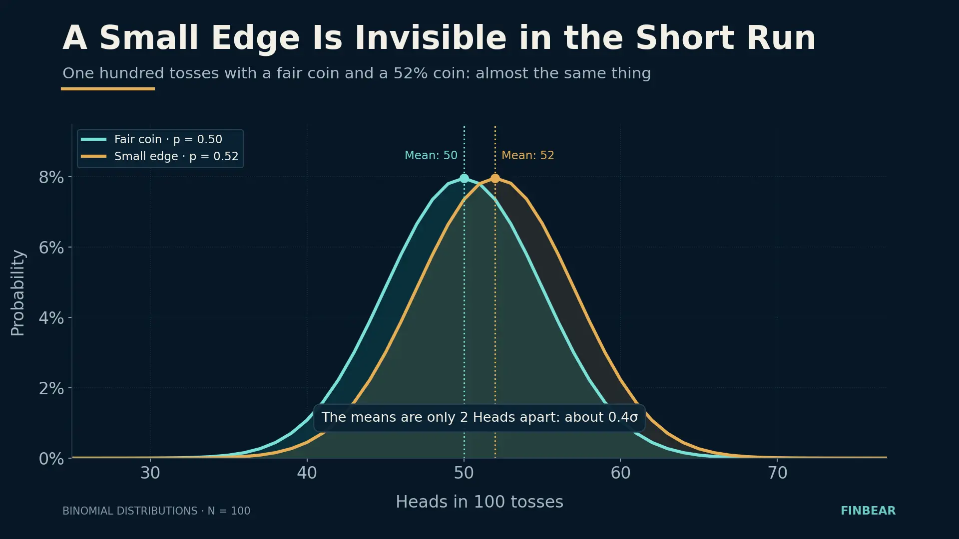
If $p > 0.5$ the walk has positive drift. If $p < 0.5$, negative. If $p = 0.5$, no preferred direction.

That gap from 50% is the most elementary form of statistical edge. And it’s all you need: not certainty, not being right every time. A small, persistent gap.

But don’t confuse edge with profit, because they’re two different things and the difference kills portfolios. A method that wins 40% of the time can be excellent if it makes three times as much when it’s right as it loses when it’s wrong. A method that wins 70% can be a disaster if the three losses in ten are enormous. The edge doesn’t live in the frequency of wins: it lives in the product of probability and size of outcomes, net of costs.

And there’s a third term almost nobody accounts for, and it follows directly from the $\sqrt{N}$ two paragraphs back: how much you bet. A real edge, bet too big, produces ruin with probability one. That’s what John Kelly formalized in 1956 while working on noise in telephone lines, and what markets have rediscovered one crisis at a time.

Being right, knowing what being right is worth, and staying at the table. Three things, not one.

From Steps to Percentages

The walk we’ve built so far is arithmetic: each step adds or subtracts a fixed amount. But a dollar doesn’t mean the same thing on a $10 stock and a $500 one. Prices move in percentages.

So let’s build a multiplicative model. Starting price 100 — an arbitrary base, chosen because it makes every figure readable as a percentage. At each period we draw a random number $U$ uniform between 0 and 1 — that’s just the way we simulate the toss, not a new probability: the coin is still fair, $p = 0.5$.

If $U > 0.5$ the price rises 1%. Otherwise it falls 1%.

\[S_{t+1} = S_t \times 1.01 \qquad \text{or} \qquad S_{t+1} = S_t \times 0.99\]

A hundred periods later we have a jagged path that looks like a financial chart. Run the simulation again: out comes another one, completely different, produced by identical rules.

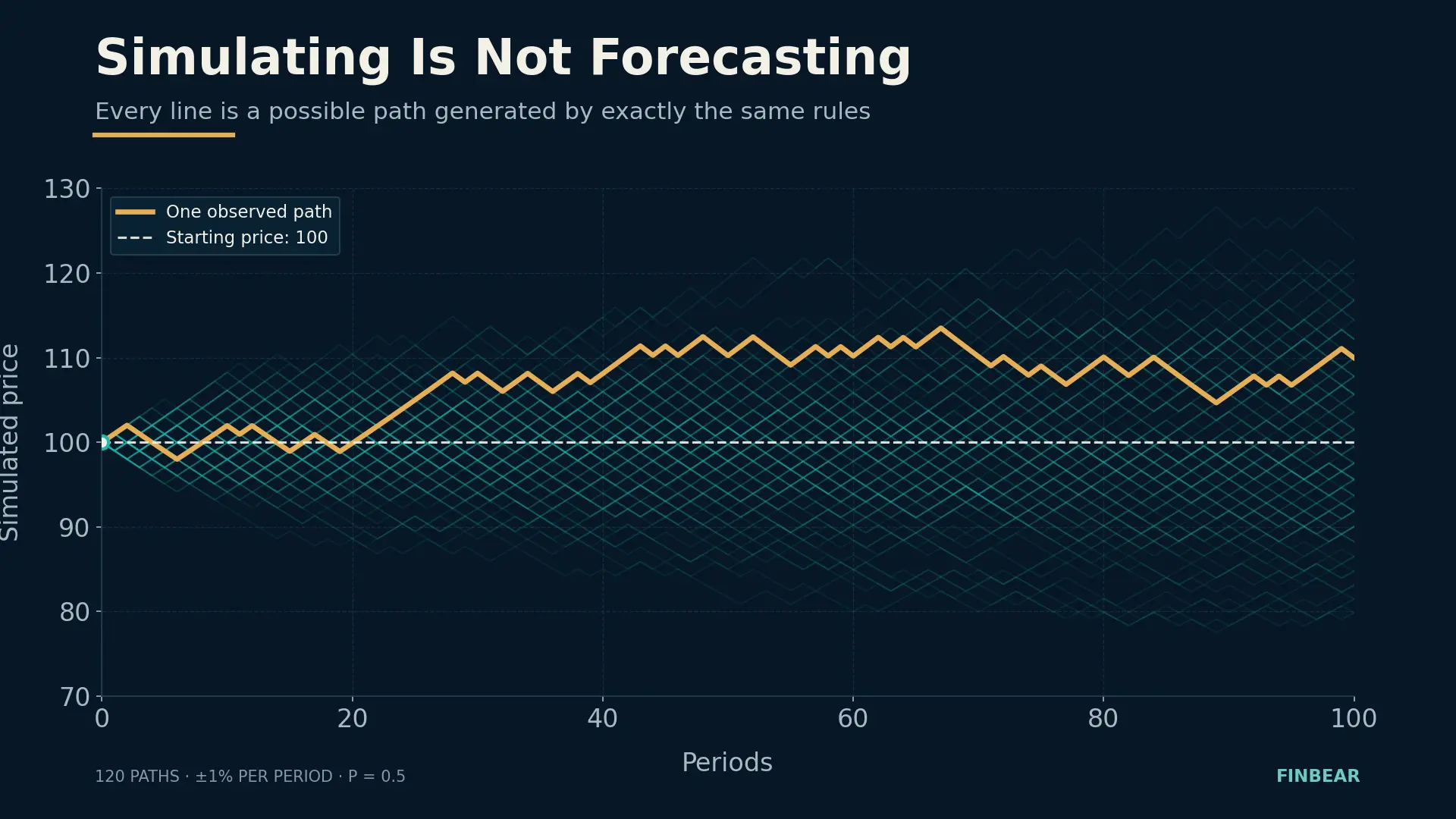
The model forecast nothing. It generated one of the paths compatible with its own rules. The chart you’re looking at isn’t the future: it’s a draw from an urn.

The +1% −1% Trap

Up 1% and then down 1% looks like a wash.

It isn’t.

\[1.01 \times 0.99 = 0.9999\]

$100 rises to $101.00 and falls to $99.99. One cent short. Looks like dust.

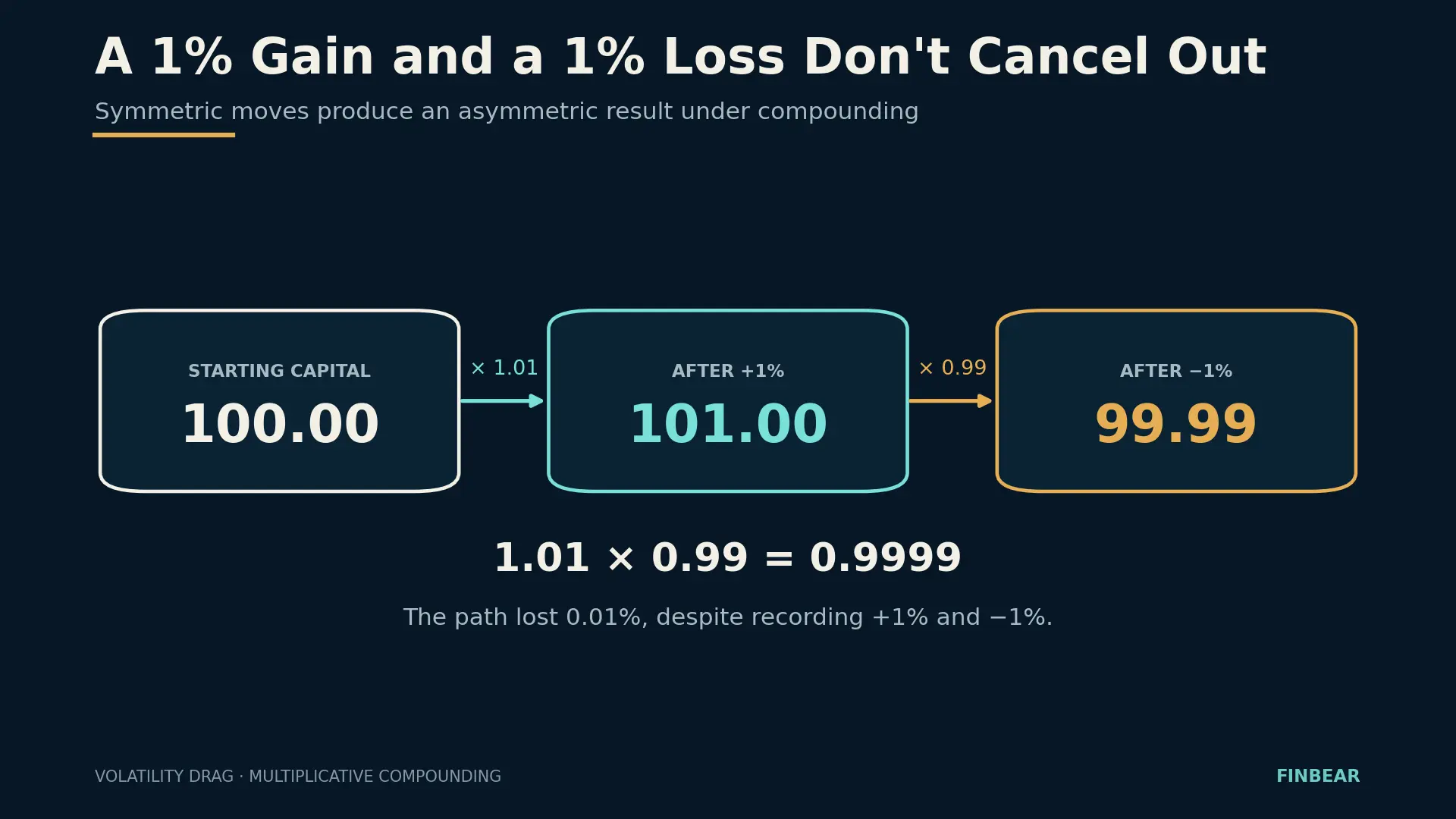
It isn’t dust, because it compounds. And here’s the arithmetic nobody runs on the model above. The arithmetic expected value of the multiplier is exactly 1:

\[0.5 \times 1.01 + 0.5 \times 0.99 = 1\]

So the expected price after 100 periods is still 100. But the median terminal value — the one reached by paths with 50 up moves and 50 down, the single most likely terminal outcome — is:

\[100 \times (1.01 \times 0.99)^{50} = 99.50\]

Mean 100. Median 99.50. The same process, two different numbers.

And the right question is: why should the second one matter?

Because the distribution of outcomes isn’t symmetric. Under multiplication, declines compress toward the floor — however much you lose, you can’t go below zero — while gains compound with no ceiling. The result is a distribution skewed to the right, with a long tail of very lucky, very rare paths. That tail pulls the mean up without moving the center.

The count can be done exactly. Over a hundred tosses, closing above 100 takes at least 51 up moves; the probability of getting them is 46%. Which means 54% of paths finish below the mean. Expected value isn’t the typical outcome: it’s a number most players never reach, held up by a minority who did far better.

And the gap widens with time. Over a thousand tosses instead of a hundred, the mean stays at 100 while the median drops to 95.12.

Hence the practical point. The arithmetic mean is the right answer to a question nobody is asking you: what would a set of a thousand parallel players get on average? That question makes sense for someone diversifying across many independent bets at the same instant. But you aren’t a thousand players: you’re one, walking a sequence of tosses one after another, and you can’t diversify across parallel copies of yourself. For someone living a path through time, the relevant statistic is compound growth along that path; in our model, the median is what a typical outcome looks like.

That’s the distinction between the ensemble average and the time average — what Ole Peters put back at the center of the debate with ergodicity economics. It isn’t academic pedantry: it’s the difference between the number in the pitch deck and the number on your statement.

This is volatility drag: volatility erodes compound growth even when it’s perfectly symmetric. You don’t need to get the direction wrong. Oscillating is enough.

It’s also why the mathematics of losses doesn’t forgive. From 100 you lose 50% and you’re at 50; you gain 50% and you’re at 75. Getting back to 100 takes 100%. Recovery is never proportional to damage, and the distance grows faster than linearly: from −20% you need +25%, from −50% you need +100%, from −80% you need +400%.

Protecting capital from large losses isn’t a personality trait. It’s arithmetic.

Where the Arithmetic Lands: μ − σ²/2

Make the steps infinitely small and the intervals infinitely short, and the random walk converges — with the right rescaling — to a continuous process: Brownian motion. The version finance uses is geometric Brownian motion:

\[dS_t = \mu S_t\,dt + \sigma S_t\,dW_t\]

where $S_t$ is the price, $\sigma$ the volatility, $dW_t$ the random shock. And $\mu$ is the expected drift — but expected of what, exactly?

Solve the equation and you find the expected price grows as $e^{\mu t}$, while the median price grows as:

\[e^{\left(\mu – \frac{\sigma^2}{2}\right)t}\]

That $-\sigma^2/2$ isn’t a technical detail. It’s the volatility drag from two paragraphs ago, written in continuous form.

Check it against our coin model, because the arithmetic lines up almost embarrassingly well. The expected simple return per period is zero, so $\mu = 0$. Its standard deviation is 0.01, so:

\[\frac{\sigma^2}{2} = \frac{0.0001}{2} = 5.0 \times 10^{-5}\]

And the expected log growth we worked out by hand:

\[\frac{\ln(1.01) + \ln(0.99)}{2} = -5.00025 \times 10^{-5}\]

Same number to four significant figures. The term that makes 100 different from 99.50 in the coin toy is the same term that shows up in the formula half the derivatives market is built on.

It’s worth knowing where all this came from, because it didn’t fall out of the sky. Louis Bachelier saw it in 1900, in Théorie de la spéculation, the thesis Poincaré examined: he applied Brownian motion to prices five years before Einstein used it for particles, and was largely ignored for half a century. Osborne picked it up in 1959, observing that what is normally distributed isn’t prices but their logarithmic changes. Samuelson carried it into modern economic form as a multiplicative process — geometric Brownian motion. From there, in 1973, Black, Scholes and Merton.

A model isn’t reality. It’s a reality simplified far enough to be interrogated.

Simulating Is Not Forecasting

Back to the uncomfortable part. A purely random process produces charts that look like markets: trends, retracements, support that holds, patterns that repeat. You can draw your lines on them and they work, because you drew them afterward.

This doesn’t prove prices are pure noise, and it doesn’t prove analysis is useless. It proves something more irritating:

A path that looks perfectly sensible can also be produced by chance.

The human brain is a pattern-finding machine with no switch to turn it off when the patterns aren’t there. It sees faces in clouds and head-and-shoulders in white noise with equal enthusiasm.

Which is why a strategy isn’t judged on a well-chosen chart. It’s judged by asking:

how many observations it rests on;
how many variants were tried before settling on that one;
what pure chance would have produced on the same sample;
whether the edge survives transaction costs;
whether it depends on three exceptional events out of two hundred;
whether it holds outside the period it was built on;
whether it stands up in a market regime different from the one it was born in.

Seven questions. None requires advanced mathematics; all of them require honesty. The reason almost nobody asks them is that four times out of five the answer kills the idea.

The second one in particular is the one nobody ever asks — and it deserves an article of its own.

Where the Model Breaks — and Why That’s the Best Part

A piece that ended here would be a dishonest piece. Because geometric Brownian motion, elegant as it is, describes real markets badly. And the ways it describes them badly are the most interesting thing in the whole story.

Real returns have fatter tails than the normal distribution allows, and not by a little. The count on $SPX from 1950 to July 2026 is brutal: across 19,257 daily log returns, the normal distribution predicts 0.011 beyond five standard deviations — in practice none, ever, in seventy-six years. There have been 53. The model is off by a factor of 4,800.

And October 19, 1987 isn’t a five-sigma session: it’s twenty-three. An event the normal curve places beyond any imaginable time scale, and which simply happened, on a Monday. Which makes the phrase “six-sigma event,” every time you hear a fund manager say it, more of a confession than a measurement.

Markets also have jumps no continuous process can generate, and volatility clustering — turbulent days calling more turbulent days, calm calling calm — while in the model every step is independent of the last. And correlations that shift precisely when you needed them stable, converging to one at exactly the moment you were counting on diversification.

Benoît Mandelbrot wrote this in 1963, studying cotton prices, and for forty years the profession preferred a wrong but tractable model to a right but inconvenient one.

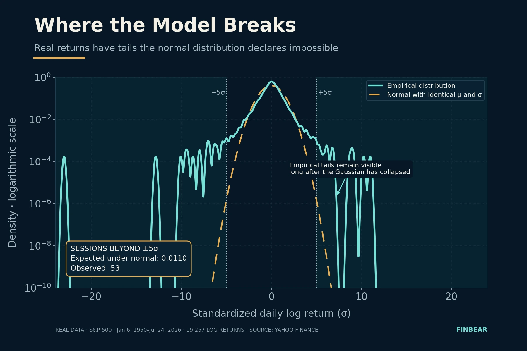
Everything else grew out of those failures: stochastic volatility models, jump processes, the GARCH family, tail risk measurement. Serious quantitative finance isn’t a defense of Brownian motion. It’s the catalogue of ways it breaks.

What FINBEAR Does With This

If the market were nothing but a fair coin, no analysis would produce a persistent edge and this site would have no reason to exist. Our job isn’t to declare that the next toss will be Heads. It’s to look for the situations where the coin might not be fair — and to measure how slightly.

With one difference that separates a coin from a market, and it’s decisive. The probability of Heads doesn’t change because somebody discovered it’s 0.5. A market anomaly, on the other hand, shrinks, mutates or disappears once enough participants find it and trade it. An edge isn’t a property: it’s a condition with an expiry date nobody tells you in advance. It has to be measured, verified and put back on trial.

In the FINBEAR method this becomes three tools doing three different jobs.

La Pythia dei Mercati draws the cone: not where the price will go, but the shape of the set of possible paths and how wide it is. It’s the dispersion chart from this article, applied to real assets. Its job is to get the single trajectory out of your head.

Quant looks for where the coin is bent. It filters a broad universe for statistical anomalies, persistent factors, asymmetries between risk and reward, recurring behavior — including the companies nobody is watching.

Istruttoria cross-examines the candidate. Because a quantitative signal doesn’t close the analysis: it opens it. Where does that edge come from, is it sustainable, what risks does the balance sheet hide, is there a verifiable catalyst — or is that number just the noise we should have expected to find, given how many places we looked.

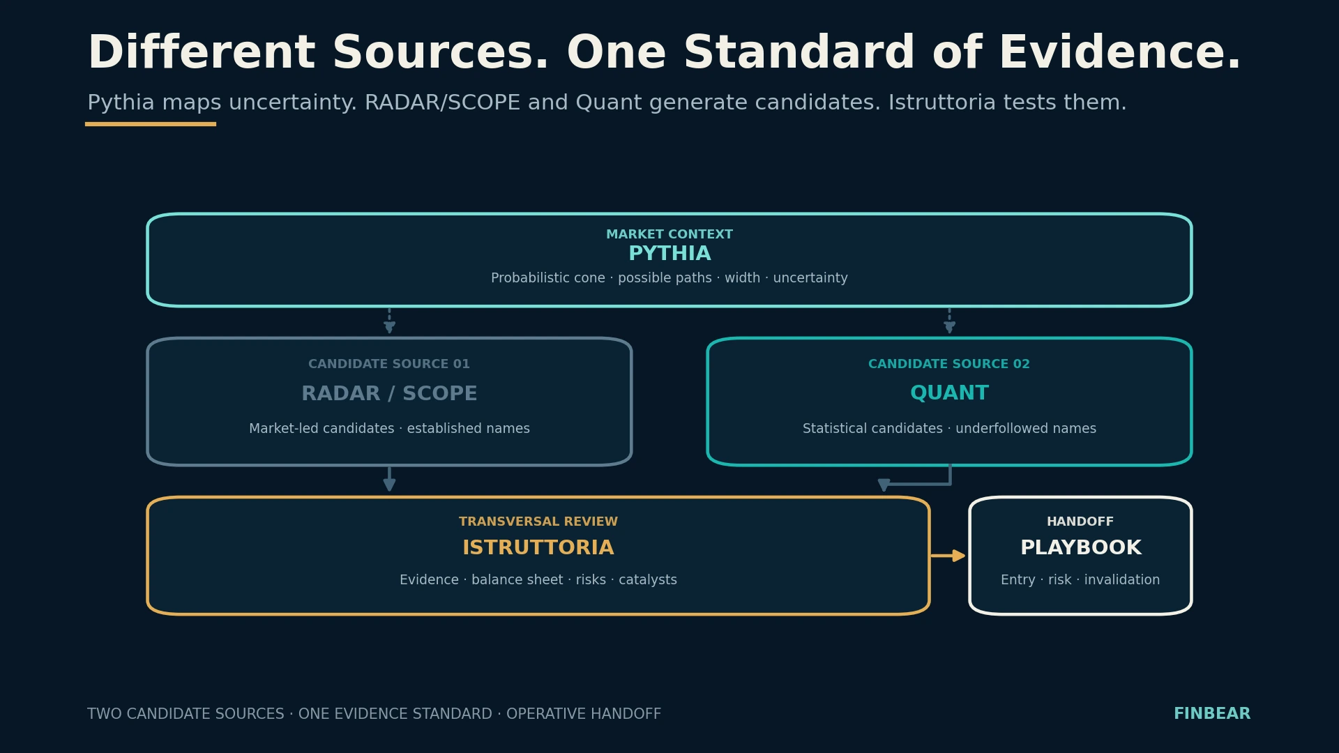
Pythia measures the uncertainty. Quant selects the case. Istruttoria examines the evidence. And the verdict, as always, is written by the price.

Don’t Guess. Measure.

The mathematics of a coin toss hands you no formula for forecasting the market. It hands you something more useful and much harder to sell.

That expected value is not the result you’ll see. That uncertainty grows even when the average stands still, and grows as the square root of time. That a tiny gap from 50% can change everything, but only if you survive long enough to watch it work. That volatility erodes compound growth even when it’s perfectly symmetric. And that a convincing chart can come from nothing at all.

The craft begins when you stop asking what will happen and start asking which outcomes are possible, with what probability, how much you can make, how much you can lose, what edge you think you have and what evidence rules out luck.

We aren’t looking for a coin that always comes up Heads. It doesn’t exist, and anyone selling you one is selling the only thing nobody owns.

We’re looking for the tables where probability, reward and risk are lopsided enough to justify a decision — and for a way of playing that keeps us seated long enough for the gap to show itself.

Understand first. Then act.

Sources

The original works behind the lineage referenced above. All are accessible; where a full version is freely available, the location is noted.

Louis Bachelier, Théorie de la spéculation, Annales scientifiques de l’École Normale Supérieure, 1900 — the thesis applying Brownian motion to prices five years before Einstein. Available on Numdam, together with Poincaré’s examiner’s report.

M. F. M. Osborne, Brownian Motion in the Stock Market, Operations Research, vol. 7 no. 2, 1959 — shows that what is normally distributed is not prices but their logarithmic changes.

Paul A. Samuelson, Rational Theory of Warrant Pricing, Industrial Management Review, 1965 — brings the multiplicative process into modern economic form.

Benoît Mandelbrot, The Variation of Certain Speculative Prices, The Journal of Business, 1963 — the cotton price study documenting fat tails forty years before the profession took them seriously.

J. L. Kelly Jr., A New Interpretation of Information Rate, Bell System Technical Journal, 1956 — the sizing criterion born out of studying noise on transmission channels.

Fischer Black and Myron Scholes, The Pricing of Options and Corporate Liabilities, Journal of Political Economy, 1973, and Robert C. Merton, Theory of Rational Option Pricing, Bell Journal of Economics and Management Science, 1973 — two distinct papers from the same year.

Ole Peters, The ergodicity problem in economics, Nature Physics, 2019, and Ole Peters and Murray Gell-Mann, Evaluating gambles using dynamics, Chaos, 2016 — the distinction between ensemble average and time average.

Data behind the tails chart: daily history of the $SPX index from January 6, 1950 to July 24, 2026, 19,257 logarithmic returns. Counts recalculated independently.

📜 Disclaimer & Fantiborsa™ Maxim

🛡️ FINBEAR™ Disclaimer:

This article is educational material. It is not investment advice, it is not a solicitation, and it is not a forecast — a word we just spent two thousand characters dismantling, so it would be rude to smuggle it back into the legal notes. If, having read that expected value is not the result you’ll see, you still decide to put eighty percent of your capital into a single idea, the problem isn’t the mathematics: the mathematics warned you. No FINBEAR content will ever tell you how the next coin lands. We teach you to estimate how bent it is, what being wrong costs you, and how much you can put on the table and still be seated at toss number one hundred. The rest you sign yourself. The verdict is written by the price.

🎭 Fantiborsa Maxim™:

“You don’t need to know how the coin lands. You need to know whether you can afford to toss it again.”